Introduction
Data-Model joint distribution is exactly process that we engineers find a model fitting beyond what we have in sampling data
“数据-模型”的联合分布,恰恰使我们工程师寻找, 一个不仅仅是, 能够拟合采样数据的模型。
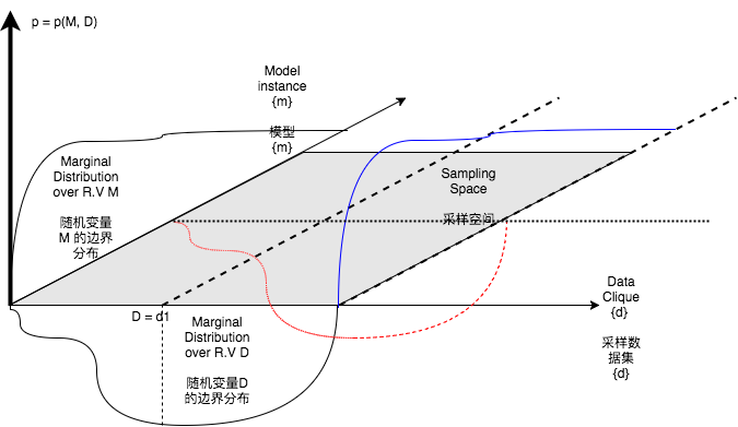
Figure1 shows how marginal distribution and joint distribution affected our sampling data and corresponding learned model. Our first approach is to discuss bases of generalization of a supervised or semisupervised model from bayesian perpectives. The bayesian perpective estimates how good a model achieved from sampled data should be. Then we dive into a specific approach widely employed by researchers and engineers in daily work -- Batched SGD. We use randomness metrics to uncover the true properties of randomness that potentially weaken our generalization.
图1 展示了边界分布,和联合分布如何影响我们的采样数据,以及从采样数据中学到的模型。本文第一个方法是,从贝叶斯角度,讨论影响监督和半监督模型的泛化因子。从贝叶斯的角度告,得知,针对采样数据学习得到的模型,到底应该多好才可以。然后我们具体的研究一个广泛采用的泛化方法,--数据桶化的随机梯度下降法。我们采用了随机性指标,揭示
To this end, we present a future model construction methodology we are working on which might achieve state of the art in the future.
末尾,我们提了下,我们正在研究一个未来的构建方法,它极有可能成为领先的模型构造方法
Basics of generalization of a model along data set
Researchers use “VC demension model” in Vladimir Vapnik and Alexey Chervonenkis’s paper published in 1971 to describe the relationship between hypothetical function and maximum sampling instances. This is becoming dramatically important especially when we have gorwing number of data. However, the concept of VC demension is weakened to some extend by the fact that modern hypothetic function is complex enough to leverage its both variation erorr and bias error for extremely large set of data,dispite that corss validation, A/B test still predominates.
研究人员, 使用VC维模型来1971 两位俄罗斯数学家的样本收敛性研究 描述“假设函数”和最大采样数据的关系。这个变得越来越重要尤其是我们的数据持续增长。然而, 由于我们的假设函数足够复杂,来均摊variance和bias(稍后将详细描述这两个概念)。某种程度上,这些模型弱化了VC维,尽管随机采样,进行cross validation和A/B test仍然是主流。
Generlaization of a model is so important that we have to be cautious about “data flow process”.

模型的泛化能力是如此重要,以至于,搞清我们所处理的采样数据,远远比采用具体的模型,更为重要。
But, we believe that Bayesian Method itself is clear enough to tell us relationship between the learned model from sampling data and sampling space (All possible data).
Simplly tell us that given data set D, the possibility that the M assigned to m.
简单地说,给定数据集合D, 被训练出来的模型是m的概率。举个例子:
e.g: we have ten sampling D belongs to {d1, d2, …, d10}, we got models m1 9 times, m2 1 time. Then
If we already know d2 produced learned model m2 (m2 ≠ m1), we say
假定,我们已经知道d2产生模型m2了,其实就是说
For The right hand side of the equation 1, if this is a classification problem, the nominator presents multiplication of correctly detected instance ratio by a model and possibility that is a true model(joint distribution tell us that a true model must not be unique).
对于方程1,右边的表达式,如果这是一个分类问题,分子是“正确被识别的比例”乘以“它是真正模型的概率”(从联合概率分布看,这个并不一定唯一)
If we perform a uniform sampling, the denomitor should always be a constant, which means
如果我们采用均匀采样,那么分母就是常数了。
When m is a random variable (we are in the learning process), the formula above requires us that prediction for the current data set might not need to be the best (a smaller value). While, when d is a random variable, We want P(m|d) or P(d|m) should not change too large. We call it variance.
加入学习模型本身就是个随机变量(我们在训练集上),上述公式要求我们,对当前数据集的预测,不能太好(小一点的值)。同时呢,采样得来的数据集,也是随机变量,我们希望条件概率,不要变化的太大。
Suppose we have two models, an estimated model m on dataset d, a true model m* we never touched, to measure our estimation m with respect to the sampling dataset D of size N, we have sampling variance Var(m) and sampling error Bias(m*, m). These two concepts already being well documented in a normal statistic textbook Introduction to Machine Learning.
现在我们有两个模型,一个是数据集d估计的模型m; 一个是我们从来没有见过的数据背后的模型m*。为了衡量在大小为N的采样数据集D的估计模型,我们拥有采样方差 Var(m) 以及,采样偏差(m*, m)。 这两个概念已经很好地在统计学教科书里面介绍了 Introduction to Machine Learning。
Batched sgd & data expansion
The normal process is sampling the best classifier m we computed over a sampled data set. If the variance of parameters of the m is large, we increase sampling size. People usually use bached sgd, if they use gradient descent strategy, making a model touch as large data as possible computationaly cheaper. But this mehthod didn’t solve the problem faced when we carry out validation process:
一般过程是对,在采样数据上得到局部最优模型,进行采样。如果参数模型的各项参数变换非常大,我就增加采样数据规模。人们常常使用,数据桶化的随机梯度下降法,使得模型可以在有限的计算资源接触到更广泛的模型样本。但它并没有解决问题的本质:
The variance could be large when feeding different data into a same model
对不同的数据,学出来的模型参数,或者预测结果的误差的方差会非常大。
The reason why it has typically good generalization might be the learned model are not the best estimation for each data set as we talked in the last chapter and data with less randomness.
但是为什么,它在一般情况下又好的,泛化,可能是因为,它针对每个数据集,都不是最好的结果;同时,数据的随机性比较少。
Regulization in history
Traditional regulization like Subset Selection, Ridge Regression and Lasso work as either solution scalar or feature selector.
In a matter of fact, previous papers use regulizaton both as panelty and opimizer scaler in a large scale machine learning, didn’t pay much attention to the fact that the regulization first employed by mathematicans in history when they were studying ploynomial hypothetic functions based on geometrical observation:
Suppose:
then, curve should not twist too much along data change direction (overfitting). This can be achieved by minimize the arc length of curve or overall unit tangent vector residual:
While,
Considering
Since equality can be achieved, we just minimize the maximum value:
We derive that regulization for generalization effects are equivalent to reducing curve arc length.
Stacked model and one true model
Before we talk about Randomness of data, let us disscuss first model architecture. In industry we can employ “stacked model” to resolve our problems in a more natural manner, while a large group people, believe that if a single deep learning model complex enough, it eventually equivalent to a stacked model. Then the model will be suitable for different senarios.
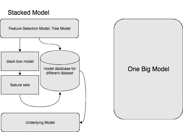
在我们讨论数据的随机性之前,我们先讨论下模型架构。在工业界,我们往往会采用“stacked model”用一种更自然的方式,去解决我们的问题。虽然我不喜欢,基于规则学习,但它确实管用。同时呢,有相当一部分人认为,只要一个训练的模型足够复杂,精巧,他们就会是等价的。而后者就可以远离业务,而移植到不同的场景中去:
Argument: Unfortunately, “Stacked models” are not equivalent to a single complex model. This argument is true especially when from one selection model like decision tree to another model (function f1 to function f2) are not uniform convergent.
论断:很遗憾,他们不会等价的。且听我道来。这个结论呢尤其是正确的,比如一个选择模型,到,另外一个模型,在相同的参数空间下,函数间不一致收敛。
Modern model solvers, in optimization theory, tightly dependence on Continuouse Differentiation Assumption. But their “differentiable definition” based on limitation theory and Not Valid For Infinite Value.
现代的求解器,在优化理论中,紧密地依赖“连续微分”假设。然而,这种基于极限的理论的定义,对于无穷变量,是没有意义的。
In arround 1930, researchers studied on Quantum Theory and Partial Differential Equation, introduced a new concept called “general differentiable” for Heaviside function. In Mathematics and Physics, Heaviside step function which is a difference of absolute value function, could be written in an integral form. In generaly differentiable case, if one can be written in an integral form, we name it generally differentiable(think about it, an integral should be differentiable right?). The theory is about density estimation just like what we do in unsupervised learning.
大概在1930年的时候,研究者在研究量子理论和偏微分方程的时候,给Heaviside函数,引进了一种新的概念,叫做“广义微分”。其实这个概念很简单。想想看,积分函数是不是一定可微分?那我把他写成积分形式,可不可以呀?当然可以。这个理论其实恰恰和我日常做得非监督学习,的密度估计,是吻合的。
Then reason why mentioned IT here is , in traditional methodology, to solve an optimization like
我为什么在这里提到它呢?这是因为,传统方法里面,要解决一下优化问题:
Solution is,discrete optimal function:
解其实是一个,离散优化函数:
These exotic points will be discarded in a large model becuase by no means they become exotic again. If consider in a general differentiable case, I am exited found that they might deeply embeded into an underlying unsupervised learning – density estimation. They participate in algorithms by no means one phase but multiple phases.
这些奇异点,在一个更大的模型里面没有理由不被抛弃,可行域不一样。 考虑一个更一般的微分问题,非常可以惊奇地发现,它们深深地嵌入底层的无监督学习 – 密度估计。
philosophy behind is: NNS, Quantile Regression based grouping methods will help us build a model database for different queries. Model database, used in hight level programming or top k mini heap selection procedure for unlinear mapping purpose.
这背后的理念是:以临近搜索,分位数回归等为基础的聚类算法,帮助我们建立一个模型数据库,以应对不同的请求。这些模型将被用到,更抽象的 优化建模 甚至 采用小顶堆的top k选择中,作为一个非线性映射关系。
Metrics to measure a model produced by data of randomness
Randomness is essentially important to success of a model. Suppose we have a query “q”, which accepted by a model m, we preform fast nearest search in dataset space hashed by its features, and found that each time we use a model to predict value, they have an error, but the E(e)≠0 > c and Var(e) is large. Noticed that the query is similar, we have following adjugement:
- Bayesian theroy assumes that we have sampling data from one truely process. The error of model measures randomness. However such randomness might come from different groups of data even though they have similar features.
- A truely random variable’s value cannot be predicted with 100% confidence. That means you might get a very small error but with confidence 0. It does nothing good for your model. This ocurr frequently for complicated data from real world.
- Gaussian Mixture Model, Quantile Regression, NNS, Density Estimation are among the most commonly used good tools to carry out Randomness research and testing
数据的随机性对于模型是非常重要的。假定我有一个查询q,作为模型m的输入,我们在分布式数据库启用快速临近搜索, 发现我们每一次预测的数值都有一个误差,并且满足 平均值不等于且大于一个常数,方差较大。注意到查询是相似样本检测,我们有以下结论:
- 贝叶斯理论,假定我们是从同一个真实却未知的随机过程采样的。误差衡量了数据的随机性。但是这样的随机性可能来自不同的数据集合,尽管他们的特征是相似的。
- 一个真正的随机变量是不可以,以置信度100%去预测的。极端地,有可能的误差非常小的,可信度是0. 这对我们的模型没有一点好处。这个在真实世界中针对复杂的业务模型,是频繁发生的。
- 混合高斯模型,分位数回归,临近搜索,和密度估计是用来检测随机性的,非常好用的工具。
For example, a model has a constant called bias which applied to all participated training samplings. Imagine it, that is nothing other than systematic error in physics like instrumental error, feature sampling error in product evironment. But empirical data, systematic error, according to my research in real projects in industry, is not simply a constant but a selection function:
比方说,模型有一个常数,叫做 bias,用于所有的参与计算的样本中。它其实和物理学中的机械等的系统误差没有区别的。但是历史数据告诉我们,这个bias可不是常数,而是一个选择函数。
Step function is not differentiable in common sense!. For truely random data, we focus on trend with specific confidence. Let me show you a concrete example to illustrate the theory.
很显然,选择函数在通常意义下不可微分。 对于真正随机的数据来说,我们应当把注意力放在置信区间上,而不是训练样本的误差。比如:
There is a company X. They want to get a model from data collected in different cities to predict how people use their products.
They found that, if they analyse in a district level, the result is evident and coinsides with the common sense; if they analyze in a city level, only few cities show significant results;
well, if you analyze in street level, the result is unpredictable and of hight variance in cross validation process, even though they could get a very small bias in training dataset because their model is complex enough.
In 2014 I wrote a simple data structure called “SeriesNode” in python to tackle above problem raised from an IoT project supported by NTU and government. As an active project manager, I was supervised by Professor Teddy from Geogia Tech.
14年的时候,我写了一个非常简单的 python 程序,叫做“SeriesNode”用来解决上述数据问题。这些问题是我参与由NTU,政府资助物联网项目的工作。作为临时项目经理,我向来自乔治亚理工的教授Teddy汇报工作。
Here is the minimum version of the codes: 这是一个最简单的代码版本:
# -*- coding: utf-8 -*-
'''
Created on 3 Nov, 2014
@author: wangyi
'''

from pandas import DataFrame, to_datetime
from core.Scheduler.delta import delta

## ---- Core Methods ----

class Node(object):

    def __init__(self, name, data):
        self.name = name
        self.data = data

        self.father = None
        self.children = list()

    def __str__(self):
        return str(self.data)

    def add_child(self, child):
        self.children.append(child)

    def add_children(self, children):
        self.children = self.children.extend(children)

    def set_children(self, children):
        self.children = children

    def set_father(self, father):
        self.father = father
        father.childer.add_child(self)

    def get_children(self):
        for child in self.children:
            print(child)
        return self.children

    def get_father(self):
        return self.father

class SeriesNode(Node):

    class seriesIterator(object):
        def __init__(self, SeriesNode, start, end, delta):
            self.SeriesNode = SeriesNode
            self.counter = self.__counter__()
            self.start = start
            self.end = end
            self.delta = delta

        def __iter__(self):
            return self

        def __counter__(self):
            start = self.start
            end   = start + self.delta
            while True:
                if  start >= self.end:
                    break
                yield (start, end)

                start = end
                end   = start + self.delta

        def __next__(self):
            try:
                start, end = next(self.counter)
                return (start, end, self.SeriesNode.data[start:end])
            except StopIteration as err:
                raise(err)

    def __init__(self, startdatetime, enddatetime, data, type='json'):
        if  type == 'json':
            ## initialization
            self.data = DataFrame(data)
            ## set index
            self.data.set_index('timestamp_utc', inplace=True)
            ## verbose
            self.data.index = to_datetime(self.data.index.astype(int), unit='s')

        elif type == 'dataframe':
            self.data = data

        super(SeriesNode, self).__init__(startdatetime.strftime("%Y%m%d%H%M"), self.data)

        self.startdatetime = startdatetime
        self.enddatetime = enddatetime
        self.treeIndex = {'monthly':[], 'weekly':[], 'dayly':[], 'daytime':[], 'nighttime':[], 'hourly':[]}

    def __iter__(self):
        return self.seriesIterator(self,
                                   self.startdatetime,
                                   self.enddatetime,
                                   self.span)

    def setup(self):
        self.treeIndex['monthly'].clear()
        self.treeIndex['weekly'].clear()
        self.treeIndex['dayly'].clear()
        self.treeIndex['daytime'].clear()
        self.treeIndex['nighttime'].clear()

        return self

        # vertical grouping
    @staticmethod
    def up2down(self, child):
        raise NotImplementedError()

    # horizontal groupign
    @staticmethod
    def left2right(self, child):
        raise NotImplementedError()

    def buildtree(self):
        raise NotImplementedError()

    def aggregate(self, obj, *callback, **keywords):
        it = self.__iter__()
        #elegant loop
        while True:
            try:
                # get data
                start, end, data = it.__next__()
                # create a child
                child = obj(start, end, data, 'dataframe', self.treeIndex)

                for call in callback:
                    call(self,
                         child
                         )

            except StopIteration as err:
                break

    def statistic(self):
        Peaks = {}
        means = None
#       stds  = None #standard deviation
        ubds  = None #unbiased deviation

        columns = self.data.columns.values

        ids = [self.data[col].idxmax() for col in columns]
        Peaks['Max'] = [self.data.loc[ids[i]][col] for i, col in enumerate(columns)]#[self.raw.loc[ids[i]][col] for i, col in enumerate(columns)]
        Peaks['Max_Time'] = [self.data.loc[ids[i]].name for i, col in enumerate(columns)]#[self.raw.loc[ids[i]]['timestamp_utc'] for i, col in enumerate(columns)]

        ids = [self.data[col].idxmin() for col in columns]
        Peaks['Min'] = [self.data.loc[ids[i]][col] for i, col in enumerate(columns)]#[self.raw.loc[ids[i]][col] for i, col in enumerate(columns)]
        Peaks['Min_Time'] = [self.data.loc[ids[i]].name for i, col in enumerate(columns)]#[self.raw.loc[ids[i]]['timestamp_utc'] for i, col in enumerate(columns)]

        means = [self.data[column].mean() for column in columns]
        ubds  = [self.data[column].std() for column in columns]

        param = {
                 'peaks':Peaks,
                 'means':means,
                 'ubds' :ubds,
                 }

        self.value = means[0]
        self.std = ubds[0]
        self.max = Peaks['Max'][0]
        self.min = Peaks['Min'][0]
        self.dt_max = Peaks['Max_Time'][0]#datetime.utcfromtimestamp(Peaks['Max_Time'][0])
        self.dt_min = Peaks['Min_Time'][0]#datetime.utcfromtimestamp(Peaks['Min_Time'][0])

        return param

## ---- Aggregation Nodes ----

class Month(SeriesNode):
    span = delta(weeks = 1)

    def __init__(self, startdatetime, enddatetime, data, type='json', treeIndex={}):
        super(Month,self).__init__(startdatetime, enddatetime, data, type=type)

        if  treeIndex != {}:
            self.treeIndex = treeIndex

        self.id = self.startdatetime.strftime("%y%m")

    def __str__(self):
        return 'Month ' + self.id + ':'

    def buildtree(self):
        self.aggregate(Week, self.up2down, self.left2right)

        return self

    # vertical grouping
    @staticmethod
    def up2down(self, child):
        self.add_child(child)
        ## up2down
        child.statistic()
        child.buildtree()

    # horizontal groupign
    @staticmethod
    def left2right(self, child):
        self.treeIndex['weekly'].append(child)
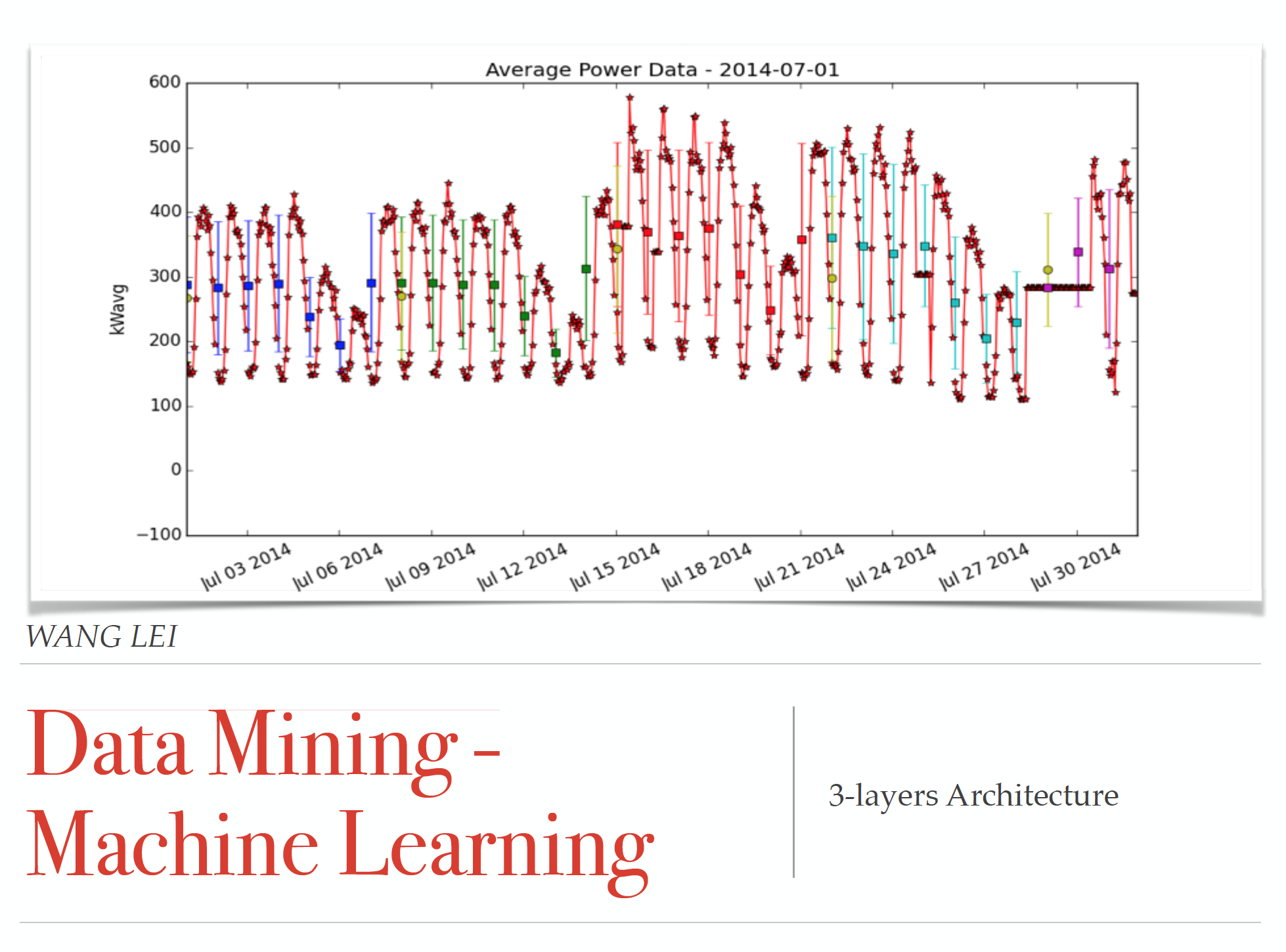
The above programme is actaully a hierarchical tree. It was initially intentionly designed as a longterm object residence in redis server to provide services of hierarchical query. As illustrated in the above pictures, we found that, data nodes in the bottom of three is of high randomness (our group collected them from meters purchased from Japan). After negotiating with the headers from Japan, we realize that the data is not instantaneous data but a data computed using mathematics from sampled data in a delta time.
上述代码,实际是一个层次树。它有意地被设计成一个长期驻扎在,redis服务器的对象,用来提供层次查询服务。如图所示,我们发现,数据在叶子节点的随机性很高!这些数据是由我们从日本采购的传感器采样得到的。在日方负责人沟通,了解到,这个数据不是瞬时数据,而是用数学公式计算得来的采样数据。
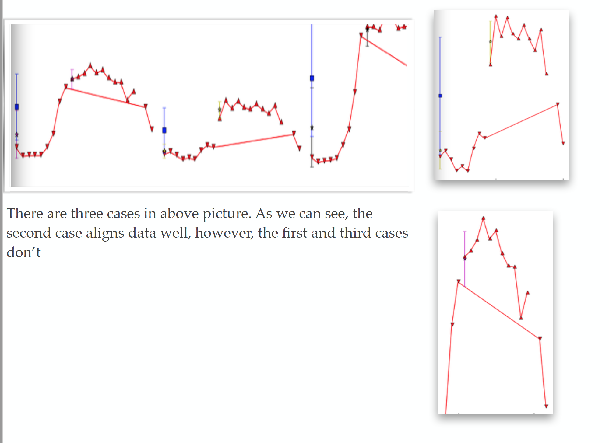
We also noticed that, at some level, the randomness tend to be eliminated at some tree depth. That means we are always doing Var prediction not Exact Value prediction. Some people challenged the idea by using a black box model for leaf nodes, while use a more explainable model in shallow depth of the data tree.
我们还注意到,在某个深度时,随机性消失了!这意味着,我们始终做基于趋势的,方差估计,而非点值估计。某公司工作人员试图用,底层黑箱模型+上层可解释模型,挑战上述模型的有效性时,我提问,“您的模型是不是在大的数据分类时,泛化能力准;在细节数据上泛化能力不准?”。对方答“是”。这就是一个随机性的很好例子。
Mapping Direction – What if bidirectional mapping?
This is a very important work I am currently working on based on my work in 2014 when I was doing an internship in I2R supervised by Senior Scientist Huang Dongyan. Simply put, typically researchers working on a mapping F from samping space X to target space Y, and use minimun error or minimum distance to supvise learning. We are comparing data in the similar target sampling space.
Should we design a model m1 mapping X to Sapce U, and model m2 mapping Y to space V? We don’t requre U, V are from the same samping space. We just require they being of similar demisions and supvise the learning using Maximum Correlation. And if m2 is invertible, we can built mapping from X to Y using m1(m2)-1. Shall we see.
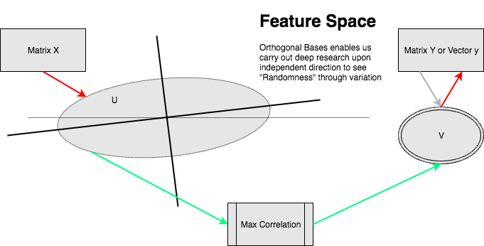
The purpose we discusss the methedology here is to support Generalization in Randomness Perpectives analysis because randomness in independant component is much easier to observe. Also, mapping features to a new space, we usually get a better aggregation result -- Spectral Clustering.
Traditional form of ml cost is:
If L(•,•) defined as an inner product over two sample spaces, we can also write it as
Where,
The general form of ml cost function can be hereby written in another form:
CCA and PLSR use the similiar form. But they are limited to a least square regression to connect to multiple responses under a simple error assumption:
Such an assumption might not be pragmatic in current application. We already know non-linear hypothetic function has stronger abilit to fit than traditional models, and we should combine to see what exiting models we can achieve towards a more theoretically high generalization. Instead we assume that true responses of the form:
Randomness Measured by Variation in Independent Component Direction
Design Pattern:
Algorithm Formulation:
Codes or theory
Experiments
Please refer to: This public address
Conclusion
Bibliography
- Vapnic, V.N & Chervonenkis, A. Y. (1971), “On the uniform convergence of relative ferequncies of events to their probabilities,” Theory of Probability and Its Application XVI(2), 264-280
- Large-Scale Machine Learning for Classification and Search Wei Liu. PhD Thesis 2012.
- Ethem Alpaydin. 2010. Introduction to Machine Learning (2nd ed.). The MIT Press.
- Regression Shrinkage and Selection via the Lasso, Robert Tibshirani
- FISHER, R. A. (1936), THE USE OF MULTIPLE MEASUREMENTS IN TAXONOMIC PROBLEMS. Annals of Eugenics, 7: 179–188. doi:10.1111/j.1469-1809.1936.tb02137.x
- Dhillon, Inderjit; Yuqiang Guan; Brian Kulis (November 2007). “Weighted Graph Cuts without Eigenvectors: A Multilevel Approach”. IEEE Transactions on Pattern Analysis and Machine Intelligence. 29 (11): 1–14. doi:10.1109/tpami.2007.1115